pyhht package
Submodules
pyhht.emd module
Empirical Mode Decomposition.
-
pyhht.emd.EMD¶ alias of
pyhht.emd.EmpiricalModeDecomposition
-
class
pyhht.emd.EmpiricalModeDecomposition(x, t=None, threshold_1=0.05, threshold_2=0.5, alpha=0.05, ndirs=4, fixe=0, maxiter=2000, fixe_h=0, n_imfs=0, nbsym=2, bivariate_mode='bbox_center')¶ Bases:
objectThe EMD class.
Methods
decompose()Decompose the input signal into IMFs. io()Compute the index of orthoginality, as defined by: keep_decomposing()Check whether to continue the sifting operation. mean_and_amplitude(m)Compute the mean of the envelopes and the mode amplitudes. stop_EMD()Check if there are enough extrema (3) to continue sifting. stop_sifting(m)Evaluate the stopping criteria for the current mode. -
__init__(x, t=None, threshold_1=0.05, threshold_2=0.5, alpha=0.05, ndirs=4, fixe=0, maxiter=2000, fixe_h=0, n_imfs=0, nbsym=2, bivariate_mode='bbox_center')¶ Empirical mode decomposition.
Parameters: - x : array-like, shape (n_samples,)
The signal on which to perform EMD
- t : array-like, shape (n_samples,), optional
The timestamps of the signal.
- threshold_1 : float, optional
Threshold for the stopping criterion, corresponding to \(\theta_{1}\) in [3]. Defaults to 0.05.
- threshold_2 : float, optional
Threshold for the stopping criterion, corresponding to \(\theta_{2}\) in [3]. Defaults to 0.5.
- alpha : float, optional
Tolerance for the stopping criterion, corresponding to \(\alpha\) in [3]. Defaults to 0.05.
- ndirs : int, optional
Number of directions in which interpolants for envelopes are computed for bivariate EMD. Defaults to 4. This is ignored if the signal is real valued.
- fixe : int, optional
Number of sifting iterations to perform for each IMF. By default, the stopping criterion mentioned in [1] is used. If set to a positive integer, each mode is either the result of exactly fixe number of sifting iterations, or until a pure IMF is found, whichever is sooner.
- maxiter : int, optional
Upper limit of the number of sifting iterations for each mode. Defaults to 2000.
- n_imfs : int, optional
Number of IMFs to extract. By default, this is ignored and decomposition is continued until a monotonic trend is left in the residue.
- nbsym : int, optional
Number of extrema to use to mirror the signals on each side of their boundaries.
- bivariate_mode : str, optional
The algorithm to be used for bivariate EMD as described in [4]. Can be one of ‘centroid’ or ‘bbox_center’. This is ignored if the signal is real valued.
References
[1] Huang H. et al. 1998 ‘The empirical mode decomposition and the Hilbert spectrum for nonlinear and non-stationary time series analysis.’ Procedings of the Royal Society 454, 903-995 [2] Zhao J., Huang D. 2001 ‘Mirror extending and circular spline function for empirical mode decomposition method’. Journal of Zhejiang University (Science) V.2, No.3, 247-252 [3] Gabriel Rilling, Patrick Flandrin, Paulo Gonçalves, June 2003: ‘On Empirical Mode Decomposition and its Algorithms’, IEEE-EURASIP Workshop on Nonlinear Signal and Image Processing NSIP-03 [4] Gabriel Rilling, Patrick Flandrin, Paulo Gonçalves, Jonathan M. Lilly. Bivariate Empirical Mode Decomposition. 10 pages, 3 figures. Submitted to Signal Processing Letters, IEEE. Matlab/C codes and additional .. 2007. <ensl-00137611> Examples
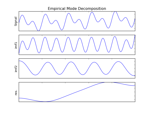
>>> from pyhht.visualization import plot_imfs
>>> import numpy as np
>>> t = np.linspace(0, 1, 1000)
>>> modes = np.sin(2 * pi * 5 * t) + np.sin(2 * pi * 10 * t)
>>> x = modes + t
>>> decomposer = EMD(x)
>>> imfs = decomposer.decompose()
>>> plot_imfs(x, imfs, t)
(Source code, png, hires.png, pdf)
Attributes: - is_bivariate : bool
Whether the decomposer performs bivariate EMD. This is automatically determined by the input value. This is True if at least one non-zero imaginary component is found in the signal.
- nbits : list
List of number of sifting iterations it took to extract each IMF.
-
decompose()¶ Decompose the input signal into IMFs.
This function does all the heavy lifting required for sifting, and should ideally be the only public method of this class.
Returns: - imfs : array-like, shape (n_imfs, n_samples)
A matrix containing one IMF per row.
Examples
>>> from pyhht.visualization import plot_imfs
>>> import numpy as np
>>> t = np.linspace(0, 1, 1000)
>>> modes = np.sin(2 * pi * 5 * t) + np.sin(2 * pi * 10 * t)
>>> x = modes + t
>>> decomposer = EMD(x)
>>> imfs = decomposer.decompose()
-
io()¶ Compute the index of orthoginality, as defined by:
\[\sum_{i,j=1,i\neq j}^{N}\frac{\|C_{i}\overline{C_{j}}\|}{\|x\|^2}\]Where \(C_{i}\) is the \(i\) th IMF.
Returns: - float
Index of orthogonality. Lower values are better.
Examples
>>> import numpy as np
>>> t = np.linspace(0, 1, 1000)
>>> modes = np.sin(2 * pi * 5 * t) + np.sin(2 * pi * 10 * t)
>>> x = modes + t
>>> decomposer = EMD(x)
>>> imfs = decomposer.decompose()
>>> print('%.3f' % decomposer.io())
0.017
-
keep_decomposing()¶ Check whether to continue the sifting operation.
-
mean_and_amplitude(m)¶ Compute the mean of the envelopes and the mode amplitudes.
Parameters: - m : array-like, shape (n_samples,)
The input array or an itermediate value of the sifting process.
Returns: - tuple
A tuple containing the mean of the envelopes, the number of extrema, the number of zero crosssing and the estimate of the amplitude of themode.
-
stop_EMD()¶ Check if there are enough extrema (3) to continue sifting.
Returns: - bool
Whether to stop further cubic spline interpolation for lack of local extrema.
-
stop_sifting(m)¶ Evaluate the stopping criteria for the current mode.
Parameters: - m : array-like, shape (n_samples,)
The current mode.
Returns: - bool
Whether to stop sifting. If this evaluates to true, the current mode is interpreted as an IMF.
-
pyhht.utils module
Utility functions used to inspect EMD functionality.
-
pyhht.utils.boundary_conditions(signal, time_samples, z=None, nbsym=2)¶ Extend a 1D signal by mirroring its extrema on either side.
Parameters: - signal : array-like, shape (n_samples,)
The input signal.
- time_samples : array-like, shape (n_samples,)
Timestamps of the signal samples
- z : array-like, shape (n_samples,), optional
A proxy signal on whose extrema the interpolation is evaluated. Defaults to signal.
- nbsym : int, optional
The number of extrema to consider on either side of the signal. Defaults to 2
Returns: - tuple
A tuple of four arrays which represent timestamps of the minima of the extended signal, timestamps of the maxima of the extended signal, minima of the extended signal and maxima of the extended signal. signal, minima of the extended signal and maxima of the extended signal.
Examples
>>> from __future__ import print_function
>>> import numpy as np
>>> signal = np.array([-1, 1, -1, 1, -1])
>>> tmin, tmax, vmin, vmax = boundary_conditions(signal, np.arange(5))
>>> tmin
array([-2,  2,  6])
>>> tmax
array([-3, -1,  1,  3,  5,  7])
>>> vmin
array([-1, -1, -1])
>>> vmax
array([1, 1, 1, 1, 1, 1])
-
pyhht.utils.extr(x)¶ Extract the indices of the extrema and zero crossings.
Parameters: - x : array-like, shape (n_samples,)
Input signal.
Returns: - tuple
A tuple of three arrays representing the minima, maxima and zero crossings of the signal respectively.
Examples
>>> from __future__ import print_function
>>> import numpy as np
>>> x = np.array([0, -2, 0, 1, 3, 0.5, 0, -1, -1])
>>> indmin, indmax, indzer = extr(x)
>>> print(indmin)
[1]
>>> print(indmax)
[4]
>>> print(indzer)
[0 2 6]
-
pyhht.utils.get_envelops(x, t=None)¶ Get the upper and lower envelopes of an array, as defined by its extrema.
Parameters: - x : array-like, shape (n_samples,)
The input array.
- t : array-like, shape (n_samples,), optional
Timestamps of the signal. Defaults to np.arange(n_samples,)
Returns: - tuple
A tuple of arrays representing the upper and the lower envelopes respectively.
Examples
>>> import numpy as np
>>> x = np.random.rand(100,)
>>> upper, lower = get_envelops(x)
-
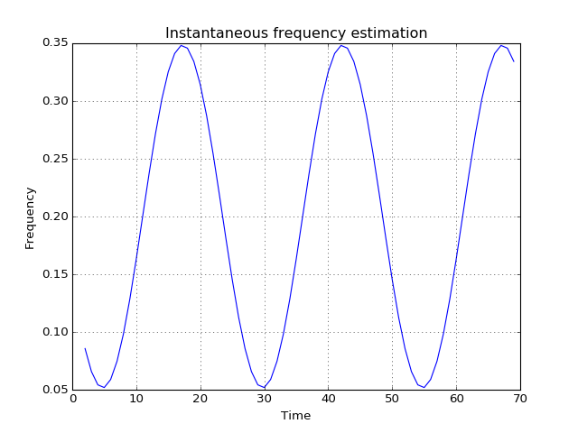
pyhht.utils.inst_freq(x, t=None)¶ Compute the instantaneous frequency of an analytic signal at specific time instants using the trapezoidal integration rule.
Parameters: - x : array-like, shape (n_samples,)
The input analytic signal.
- t : array-like, shape (n_samples,), optional
The time instants at which to calculate the instantaneous frequency. Defaults to np.arange(2, n_samples)
Returns: - array-like
Normalized instantaneous frequencies of the input signal
Examples
>>> from tftb.generators import fmsin
>>> import matplotlib.pyplot as plt
>>> x = fmsin(70, 0.05, 0.35, 25)[0]
>>> instf, timestamps = inst_freq(x)
>>> plt.plot(timestamps, instf)
(Source code, png, hires.png, pdf)
pyhht.visualization module
Visualization functions for PyHHT.
-
pyhht.visualization.plot_imfs(signal, imfs, time_samples=None, fignum=None, show=True)¶ Plot the signal, IMFs and residue.
Parameters: - signal : array-like, shape (n_samples,)
The input signal.
- imfs : array-like, shape (n_imfs, n_samples)
Matrix of IMFs as generated with the EMD.decompose method.
- time_samples : array-like, shape (n_samples), optional
Time instants of the signal samples. (defaults to np.arange(1, len(signal)))
- fignum : int, optional
Matplotlib figure number (by default a new figure is created)
- show : bool, optional
Whether to display the plot. Defaults to True, set to False if further plotting needs to be done.
Returns: - `matplotlib.figure.Figure`
The figure (new or existing) in which the decomposition is plotted.
Examples
>>> from pyhht.visualization import plot_imfs
>>> import numpy as np
>>> from pyhht import EMD
>>> t = np.linspace(0, 1, 1000)
>>> modes = np.sin(2 * np.pi * 5 * t) + np.sin(2 * np.pi * 10 * t)
>>> x = modes + t
>>> decomposer = EMD(x)
>>> imfs = decomposer.decompose()
>>> plot_imfs(x, imfs, t)
(Source code, png, hires.png, pdf)
Module contents
-
pyhht.EMD¶ alias of
pyhht.emd.EmpiricalModeDecomposition
-
class
pyhht.EmpiricalModeDecomposition(x, t=None, threshold_1=0.05, threshold_2=0.5, alpha=0.05, ndirs=4, fixe=0, maxiter=2000, fixe_h=0, n_imfs=0, nbsym=2, bivariate_mode='bbox_center')¶ Bases:
objectThe EMD class.
Methods
decompose()Decompose the input signal into IMFs. io()Compute the index of orthoginality, as defined by: keep_decomposing()Check whether to continue the sifting operation. mean_and_amplitude(m)Compute the mean of the envelopes and the mode amplitudes. stop_EMD()Check if there are enough extrema (3) to continue sifting. stop_sifting(m)Evaluate the stopping criteria for the current mode. -
__init__(x, t=None, threshold_1=0.05, threshold_2=0.5, alpha=0.05, ndirs=4, fixe=0, maxiter=2000, fixe_h=0, n_imfs=0, nbsym=2, bivariate_mode='bbox_center')¶ Empirical mode decomposition.
Parameters: - x : array-like, shape (n_samples,)
The signal on which to perform EMD
- t : array-like, shape (n_samples,), optional
The timestamps of the signal.
- threshold_1 : float, optional
Threshold for the stopping criterion, corresponding to \(\theta_{1}\) in [3]. Defaults to 0.05.
- threshold_2 : float, optional
Threshold for the stopping criterion, corresponding to \(\theta_{2}\) in [3]. Defaults to 0.5.
- alpha : float, optional
Tolerance for the stopping criterion, corresponding to \(\alpha\) in [3]. Defaults to 0.05.
- ndirs : int, optional
Number of directions in which interpolants for envelopes are computed for bivariate EMD. Defaults to 4. This is ignored if the signal is real valued.
- fixe : int, optional
Number of sifting iterations to perform for each IMF. By default, the stopping criterion mentioned in [1] is used. If set to a positive integer, each mode is either the result of exactly fixe number of sifting iterations, or until a pure IMF is found, whichever is sooner.
- maxiter : int, optional
Upper limit of the number of sifting iterations for each mode. Defaults to 2000.
- n_imfs : int, optional
Number of IMFs to extract. By default, this is ignored and decomposition is continued until a monotonic trend is left in the residue.
- nbsym : int, optional
Number of extrema to use to mirror the signals on each side of their boundaries.
- bivariate_mode : str, optional
The algorithm to be used for bivariate EMD as described in [4]. Can be one of ‘centroid’ or ‘bbox_center’. This is ignored if the signal is real valued.
References
[1] Huang H. et al. 1998 ‘The empirical mode decomposition and the Hilbert spectrum for nonlinear and non-stationary time series analysis.’ Procedings of the Royal Society 454, 903-995 [2] Zhao J., Huang D. 2001 ‘Mirror extending and circular spline function for empirical mode decomposition method’. Journal of Zhejiang University (Science) V.2, No.3, 247-252 [3] Gabriel Rilling, Patrick Flandrin, Paulo Gonçalves, June 2003: ‘On Empirical Mode Decomposition and its Algorithms’, IEEE-EURASIP Workshop on Nonlinear Signal and Image Processing NSIP-03 [4] Gabriel Rilling, Patrick Flandrin, Paulo Gonçalves, Jonathan M. Lilly. Bivariate Empirical Mode Decomposition. 10 pages, 3 figures. Submitted to Signal Processing Letters, IEEE. Matlab/C codes and additional .. 2007. <ensl-00137611> Examples
>>> from pyhht.visualization import plot_imfs
>>> import numpy as np
>>> t = np.linspace(0, 1, 1000)
>>> modes = np.sin(2 * pi * 5 * t) + np.sin(2 * pi * 10 * t)
>>> x = modes + t
>>> decomposer = EMD(x)
>>> imfs = decomposer.decompose()
>>> plot_imfs(x, imfs, t)
(Source code, png, hires.png, pdf)
Attributes: - is_bivariate : bool
Whether the decomposer performs bivariate EMD. This is automatically determined by the input value. This is True if at least one non-zero imaginary component is found in the signal.
- nbits : list
List of number of sifting iterations it took to extract each IMF.
-
decompose()¶ Decompose the input signal into IMFs.
This function does all the heavy lifting required for sifting, and should ideally be the only public method of this class.
Returns: - imfs : array-like, shape (n_imfs, n_samples)
A matrix containing one IMF per row.
Examples
>>> from pyhht.visualization import plot_imfs
>>> import numpy as np
>>> t = np.linspace(0, 1, 1000)
>>> modes = np.sin(2 * pi * 5 * t) + np.sin(2 * pi * 10 * t)
>>> x = modes + t
>>> decomposer = EMD(x)
>>> imfs = decomposer.decompose()
-
io()¶ Compute the index of orthoginality, as defined by:
\[\sum_{i,j=1,i\neq j}^{N}\frac{\|C_{i}\overline{C_{j}}\|}{\|x\|^2}\]Where \(C_{i}\) is the \(i\) th IMF.
Returns: - float
Index of orthogonality. Lower values are better.
Examples
>>> import numpy as np
>>> t = np.linspace(0, 1, 1000)
>>> modes = np.sin(2 * pi * 5 * t) + np.sin(2 * pi * 10 * t)
>>> x = modes + t
>>> decomposer = EMD(x)
>>> imfs = decomposer.decompose()
>>> print('%.3f' % decomposer.io())
0.017
-
keep_decomposing()¶ Check whether to continue the sifting operation.
-
mean_and_amplitude(m)¶ Compute the mean of the envelopes and the mode amplitudes.
Parameters: - m : array-like, shape (n_samples,)
The input array or an itermediate value of the sifting process.
Returns: - tuple
A tuple containing the mean of the envelopes, the number of extrema, the number of zero crosssing and the estimate of the amplitude of themode.
-
stop_EMD()¶ Check if there are enough extrema (3) to continue sifting.
Returns: - bool
Whether to stop further cubic spline interpolation for lack of local extrema.
-
stop_sifting(m)¶ Evaluate the stopping criteria for the current mode.
Parameters: - m : array-like, shape (n_samples,)
The current mode.
Returns: - bool
Whether to stop sifting. If this evaluates to true, the current mode is interpreted as an IMF.
-
-
pyhht.plot_imfs(signal, imfs, time_samples=None, fignum=None, show=True)¶ Plot the signal, IMFs and residue.
Parameters: - signal : array-like, shape (n_samples,)
The input signal.
- imfs : array-like, shape (n_imfs, n_samples)
Matrix of IMFs as generated with the EMD.decompose method.
- time_samples : array-like, shape (n_samples), optional
Time instants of the signal samples. (defaults to np.arange(1, len(signal)))
- fignum : int, optional
Matplotlib figure number (by default a new figure is created)
- show : bool, optional
Whether to display the plot. Defaults to True, set to False if further plotting needs to be done.
Returns: - `matplotlib.figure.Figure`
The figure (new or existing) in which the decomposition is plotted.
Examples
>>> from pyhht.visualization import plot_imfs
>>> import numpy as np
>>> from pyhht import EMD
>>> t = np.linspace(0, 1, 1000)
>>> modes = np.sin(2 * np.pi * 5 * t) + np.sin(2 * np.pi * 10 * t)
>>> x = modes + t
>>> decomposer = EMD(x)
>>> imfs = decomposer.decompose()
>>> plot_imfs(x, imfs, t)
(Source code, png, hires.png, pdf)