Motivation for Hilbert Spectral Analysis
The Fourier transform generalizes Fourier coefficients of a signal over time. Since the Fourier coefficients are the measures of the signal amplitude as a function of frequency, the time information is totally lost, as we saw in the last section. To address this issue there have developed further modifications of the Fourier transform, the most popular of which is the short-time Fourier transform (STFT). The STFT divides the input signal into windows of time and then considers the Fourier transforms of those time windows, thereby achieving some localization of frequency information along the time axis. While practically powerful for most signals, this method cannot be generalized for a broad class of signals because of its a priori window lengths. Particularly, the window lengths must be long enough to capture at least one cycle of a component frequency, but not so long as to be redundant. On the other hand, most real-life signals are nonstationary, or have multiple frequency components. The duration of the STFT windows should not be so long as to mix the multiple components during a single operation of the kernel. This might lead to highly undesirable results like the frequency analysis representing multiple components of a nonstationary signal as harmonics of lower components.
A powerful variant of the Fourier transform is the wavelet transform. By using finite-support basis functions, wavelets are able to approximate even nonstationary data. These basis functions possess most of the desirable properties required for linear decomposition (like orthogonality, completeness , etc) and they can be drawn from a large dictionary of wavelets. This makes the wavelet transform a versatile tool for analysis of nonstationary data. But the wavelet transform is still a linear decomposition and hence suffers from related problems like the uncertainty principle. Moreover, like Fourier, the wavelet transform too is non-adaptive. The basis functions are selected a priori and consequently make the wavelet decomposition prone to spurious harmonics and ultimately incorrect interpretations of the data.
A remarkable advantage of Fourier based methods is their mathematical framework. Fourier based methods are so elegant that they make building models for a given dataset very easy. Although such models can represent most of the data and are extensive enough for a practical application, the fact remains that there is some amount of data slipping through the gaps left behind by linear approximations. Despite all these shortcomings, wavelet analysis still remains the best possible method for analysis of nonstationary data, and hence should be used as a reference to establish the validity of other methods.
1. The Uncertainty Principle
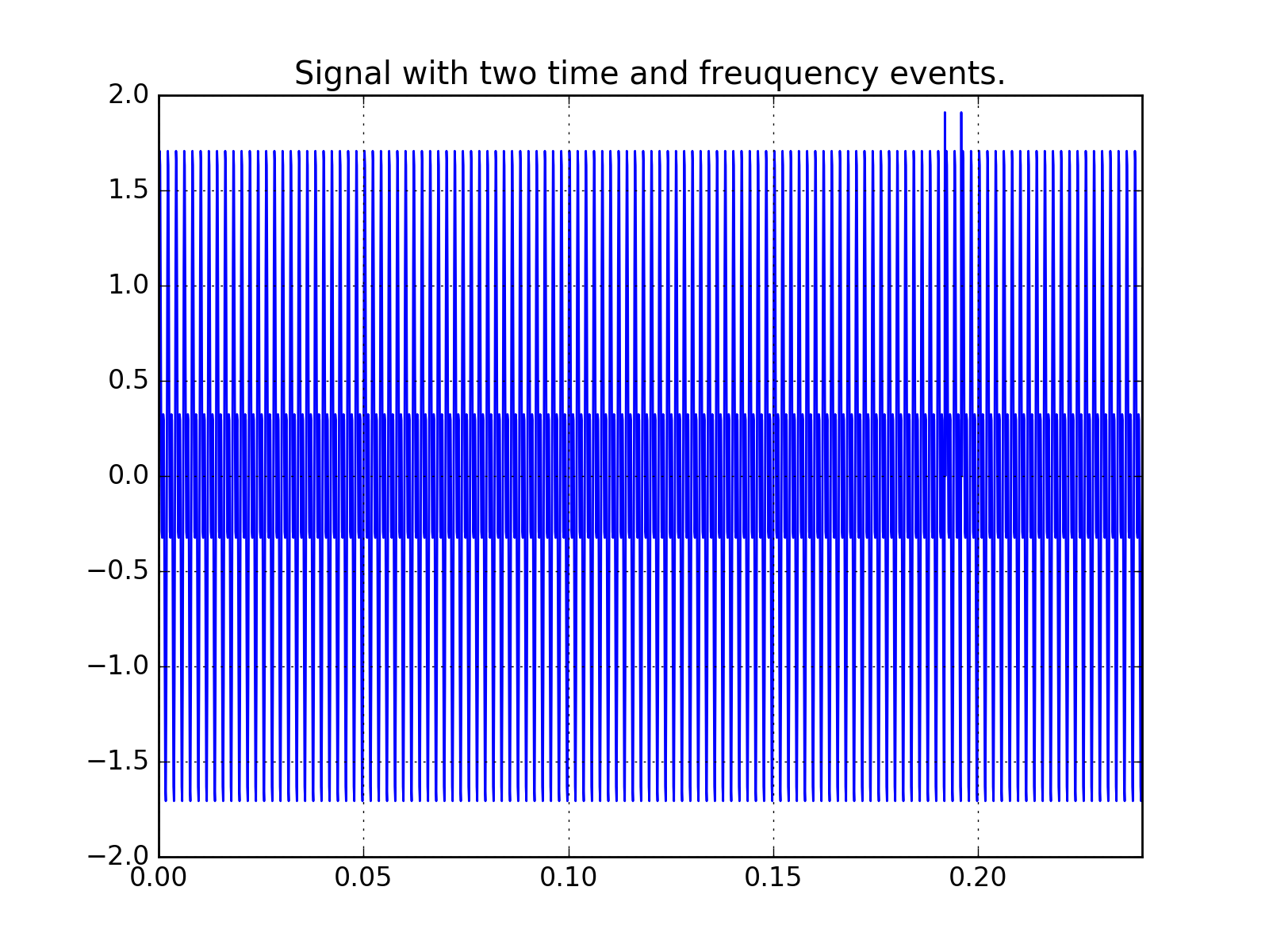
A very manifest limitation of the Fourier transform can be seen as the uncertainty principle. Consider the signal shown here:
>>> import numpy as np
>>> import matplotlib.pyplot as plt
>>> f1, f2 = 500, 1000
>>> t1, t2 = 0.192, 0.196
>>> f_sample = 8000
>>> n_points = 2048
>>> ts = np.arange(n_points, dtype=float) / f_sample
>>> signal = np.sin(2 * np.pi * f1 * ts) + np.sin(2 * np.pi * f2 * ts)
>>> signal[int(t1 * f_sample) - 1] += 3
>>> signal[int(t2 * f_sample) - 1] += 3
>>> plt.plot(ts, signal)
(Source code, png, hires.png, pdf)
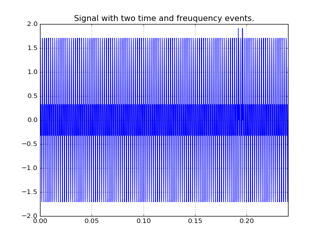
It is a sum of two sinusiodal signals of frequencies 500 Hz and 1000 Hz. It has two spikes at t = 0.192s and t = 0.196s. The purpose of a time frequency distribution would be to clearly identify both the frequencies and both the spikes, thus resolving events in both frequency and time. Let’s check out the spectrograms of the STFTs of the signal with four different window lengths:
(Source code, png, hires.png, pdf)
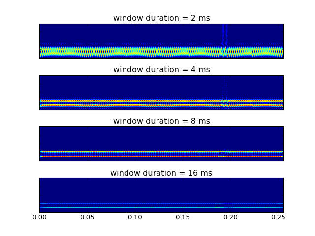
As can be clearly seen, resolution in time and frequency cannot be obtained simultaneously. In the last (bottom) image, where the window length is high, the STFT manages to discriminate between frequencies of 500 Hz and 1000 Hz very clearly, but the time resolution between the events at t = 0.192 s and t = 0.196 s is ambiguous. As we reduce the length of the window function, the resolution between the time events goes on becoming better, but only at the cost of resolution in frequencies.
This phenomenon is called the Uncertainty principle. Informally, it states that arbitrarily high resolution cannot be obtained in both time and frequency. This is a consequence of the definition of the Fourier transform. The definition insists that a signal be represented as a weighted sum of sinusoids, and therefore identifies frequency information that is globally prevalent. As a workaround to this interpretation, we use the STFT which performs the Fourier transform on limited periods of the signals. But unfortunately the period length is defined a priori, thereby making the results uncertain in either frequency or time. Mathematically this uncertainty can be quantified with the Heisenberg-Gabor Inequality (also sometimes called the Gabor limit):
Heisenberg - Gabor Inequality
If \(T\) and \(B\) are standard deviations of the time characteristics and the bandwidth respectively of a signal \(s(t)\), then
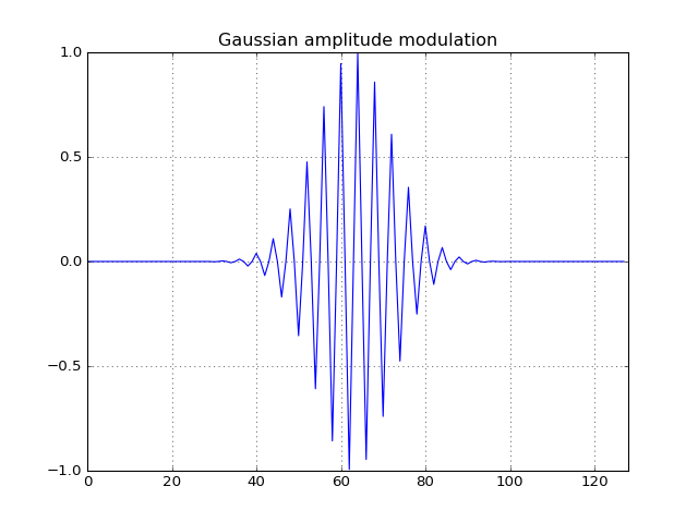
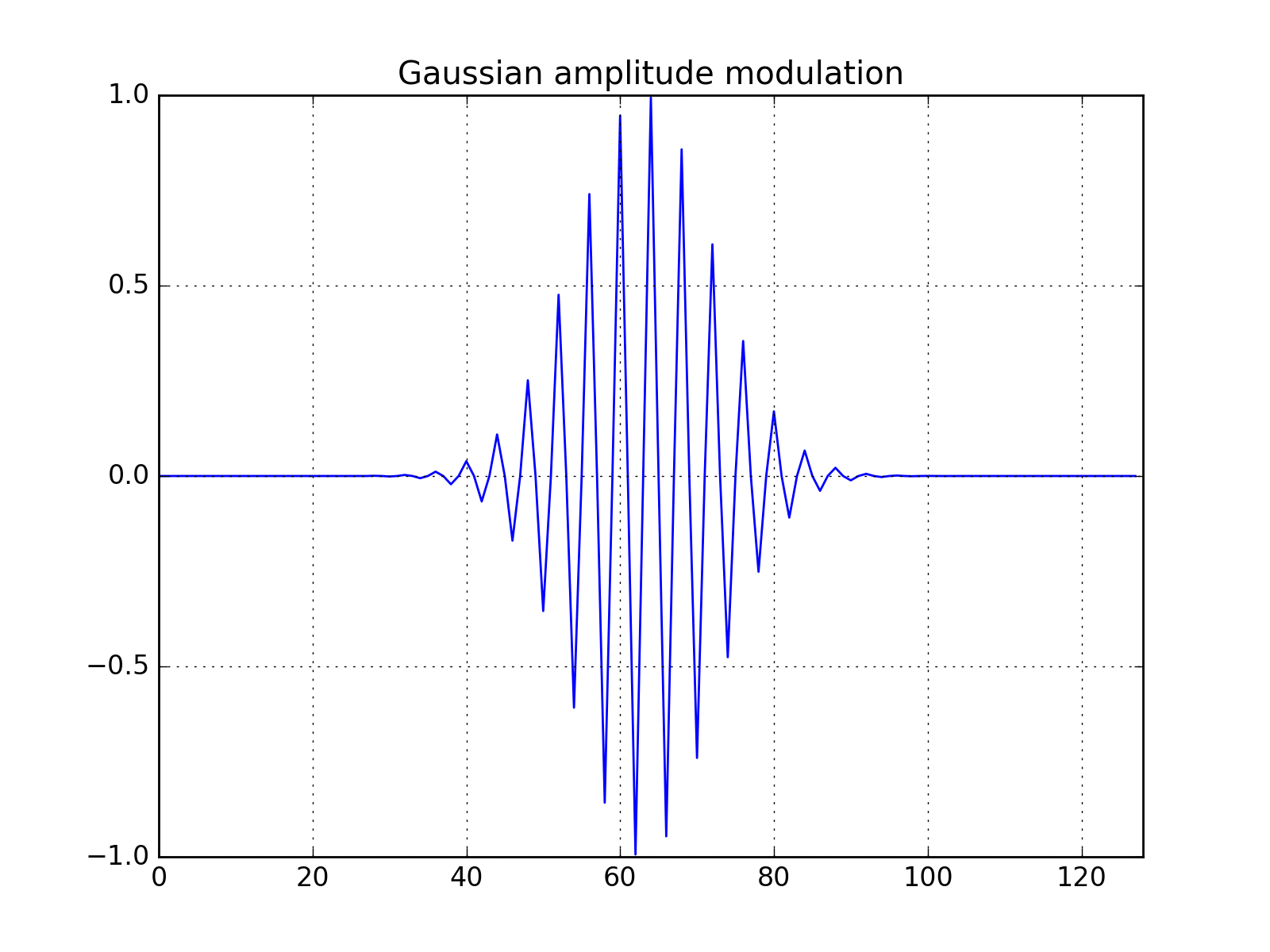
The expression states that the time-bandwidth product of a signal is lower bounded by unity. Gaussian functions satisfy the equality condition in the equation. This can be verified as follows:
>>> from tftb.generators import fmconst, amgauss
>>> x = gen.amgauss(128) * gen.fmconst(128)[0]
>>> plot(real(x))
(Source code, png, hires.png, pdf)

>>> from tftb.processing import loctime, locfreq
>>> time_mean, time_duration = loctime(x)
>>> freq_center, bandwidth = locfreq(x)
>>> time_duration * bandwidth
1.0
A remarkably insightful commentary on the Uncertainty principle is provided in [1], which states that the Uncertainty principle is a statement about two variables whose associated operators do not mutually commute. This helps us apply the Uncertainty principle in signal processing in the same way as in quantum physics.
2. Instantaneous Frequency
As a workaround to the limitations imposed by the Uncertainty principle, we can define a new measure of signal characteristics called the instantaneous frequency. The definition of instantaneous frequency has remained highly controversial ever since its inception, and it is easy to see why. When something is instantaneous it is localized in time. Since time and frequency are inverse quantities, localizing frequency in time can be highly ambiguous. However, a practical definition of instantaneous frequencies is provided in [2], and is discussed in the next section.
2.1 Analytic Signals and Instantaneous Frequencies
In order to define instantaneous frequencies we must first introduce the concept of analytic signals. For any real valued signal \(x(t)\) we associate a complex valued signal \(x_{a}(t)\) defined as:
where \(\widehat{x(t)}\) is the Hilbert transform of \(x(t)\). Then the instantaneous frequency can be defined as:
2.2 Instantaneous Frequencies from HHT
The real innovation of the HHT is an iterative algorithm called the Empirical Mode Decomposition (EMD) which breaks a signal down into so-called Intrinsic Mode Functions (IMFs) which are characterized by being narrowband, nearly monocomponent and having a large time-bandwidth product. This allows the IMFs to have well-defined Hilbert transforms and consequently, physically meaningful instantaneous frequencies. In the next couple of sections we briefly describe IMFs and the algorithm, EMD, used to obtain them.
2.3 Intrinsic Mode Functions
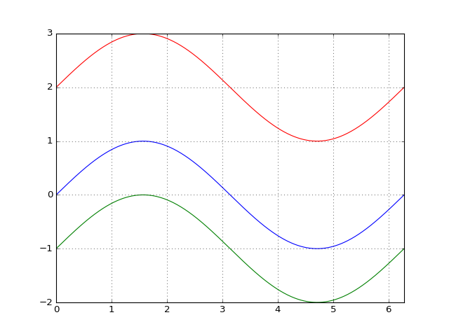
Consider the three sinusoidal signals obtained as follows:
>>> x = np.linspace(0, 2 * np.pi, 1000)
>>> s1 = np.sin(x)
>>> s2 = np.sin(x) - 1
>>> s3 = np.sin(x) + 2
>>> plt.plot(x, s1, 'b', x, s2, 'g', x, s3, 'r')
(Source code, png, hires.png, pdf)

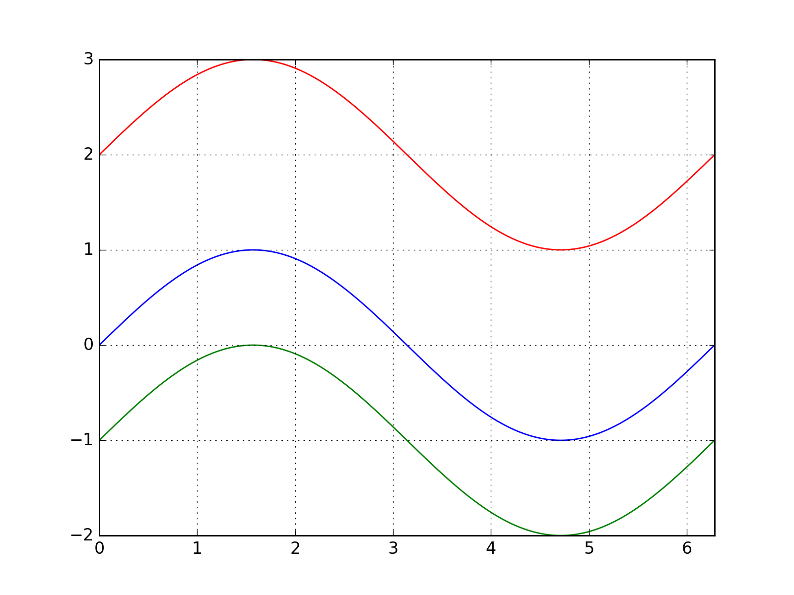
All of them are identical, except that two of them have a nonzero DC component. Since the Hilbert transform of sine is cosine, the analytic signals of these sinusoids should represent unit circles in the complex plane:
>>> from scipy.signal import hilbert
>>> hs1 = hilbert(s1)
>>> hs2 = hilbert(s2)
>>> hs3 = hilbert(s3)
>>> plt.plot(np.real(hs1), np.imag(hs1), 'b')
>>> plt.plot(np.real(hs2), np.imag(hs2), 'g')
>>> plt.plot(np.real(hs3), np.imag(hs3), 'r')
(Source code, png, hires.png, pdf)
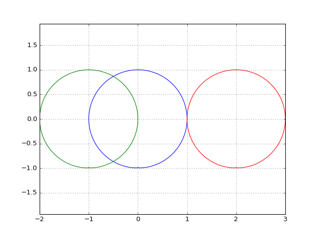
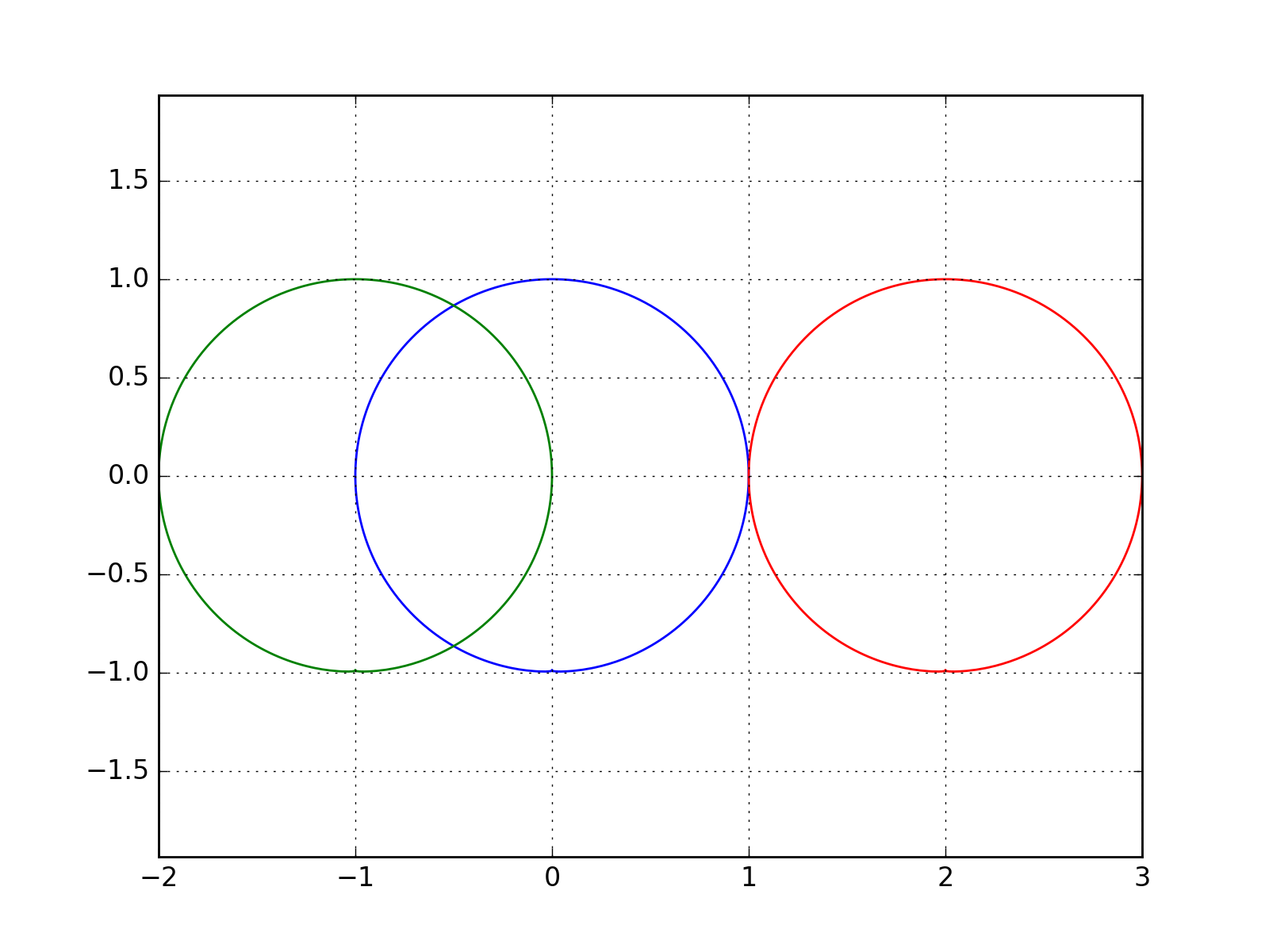
Imagine that each circle is traced out by a phasor rotating anticlockwise, which is centered at the origin in the figure above. The angle that the phasor rotates through in an infinitesimally small time period represents the instantaneous phase of the signal, and its time differential is the instantaneous frequency. Using this interpretation, let’s try to compute the instantaneous frequencies of the three signals:
>>> from scipy import angle, unwrap
>>> omega_s1 = unwrap(angle(hs1))  # unwrapped instantaneous phase
>>> omega_s2 = unwrap(angle(hs2))
>>> omega_s3 = unwrap(angle(hs3))
>>> f_inst_s1 = np.diff(omega_s1)  # instantaneous frequency
>>> f_inst_s2 = np.diff(omega_s2)
>>> f_inst_s3 = np.diff(omega_s3)
>>> plt.plot(x[1:], f_inst_s1, "b")
>>> plt.plot(x[1:], f_inst_s2, "g")
>>> plt.plot(x[1:], f_inst_s3, "r")
>>> plt.show()
(Source code, png, hires.png, pdf)

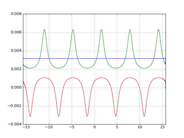
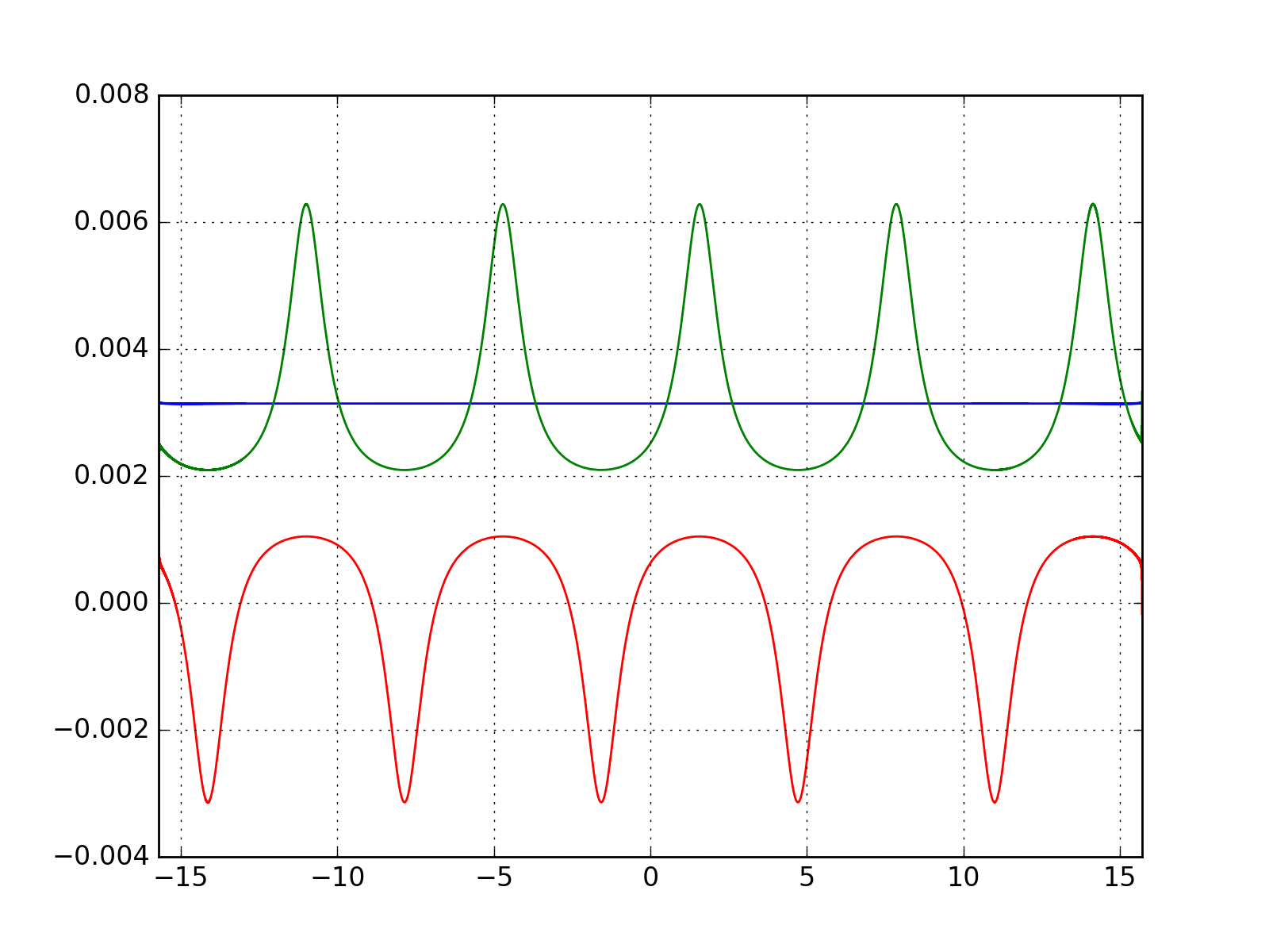
As shown in the figure, only one sinusoid presents an instantaneous frequency that is constant and corresponds to the true frequency of the waves. This wave is the one which has its analytical signal centered around the origin, thereby allowing the phasor to rotate through a total angle of 2π in one period. This is the wave that has a zero DC component and is symmetrical around the time axis.
The fact that true instantaneous frequencies are reproduced only when the signal is symmetric about the X-axis motivates the definition of an IMF.
Intrinsic Mode Functions
- A function is called an intrinsic mode function when:
- The number of its extrema and zero-crossings differ at most by unity.
- The mean of the local envelopes defined by its local maxima and that defined by its local minima should be zero at all times.
Condition 1 ensures that there are no localized oscillations in the signal and it crosses the X-axis at least once before it goes from one extremum to another, which makes it adaptive. Condition 2 ensures meaningful instantaneous frequencies, as explained in the previous example. The next section explains the algorithm for extracting IMFs out of a signal.
2.4 Empirical Mode Decomposition
The EMD is an iterative algorithm which breaks a signal down into IMFs. The process is performed as follows:
- Find all local extrema in the signal.
- Join all the local maxima with a cubic spline, creating an upper envelope. Repeat for local minima and create a lower envelope.
- Calculate the mean of the envelopes.
- Subtract mean from original signals.
- Repeat steps 1-4 until result is an IMF.
- Subtract this IMF from the original signal.
- Repeat steps 1-6 till there are no more IMFs left in the signal.
The next tutorial demonstrates how EMD can be used with PyHHT.
2.5 Properties of Intrinsic Mode Functions
By virtue of the EMD algorithm, the decomposition is complete, in that the sum of the IMFs and the residue subtracted from the input signal leaves behind only a negligible residue. The decomposition is almost orthogonal. Also, as emphasized earlier, the greatest advantage of the IMFs are well-behaved Hilbert transforms, enabling the extraction of physically meaningful instantaneous frequencies.
IMFs have large time-bandwidth products, which indicates that they tend to move away from the lower bound of the Heisenberg-Gabor inequality, thereby avoiding the limitations of the Uncertainty principle, as explained in section 1.
3. Two Views of Nonlinear Phenomena
Despite all its robustness and convenience, the Hilbert-Huang transform is unfortunately just an algorithm, without a well-defined mathematical base. All inferences drawn from it are empirical and can only be corroborated as such. It lacks the mathematical sophistication of the Fourier framework. On the plus side it provides a very realistic insight into data.
Thus here we have room for a tradeoff between the mathematical elegance of the Fourier analysis and the physical significance provided by the Hilbert-Huang transform. Wavelets are the closest thing to the HHT that not only have the ability to analyze nonlinear and nonstationary phenomena, but also a complete mathematical foundation. Unfortunately wavelets are not adaptive and as such might suffer from problems like uncertainty principle, leakages, Gibb’s phenomenon, harmonics, etc - like most of the decomposition techniques that use a priori basis functions. On the other hand, the basis functions of the HHT are IMFs which are adaptive and empirical. But EMD is not a perfect algorithm. For many signals it does not converge down to a set of finite IMFs. Some experts even believe that there is an inherent contradiction between the way IMFs are defined and the way EMD is executed. This means that we can possibly use wavelets as a ‘handle’ for the appropriate extraction of IMFs, and conversely, use IMFs to establish the physical relevance of wavelet decomposition.
Thus the Hilbert-Huang transform is a alternate view of nonlinear and nonstationary phenomena, one that is unencumbered by mathematical jargon. This lack of mathematical sophistication allows researchers to be very flexible and versatile with its use.
4. Conclusion
Consider a dark room with a photosensitive device. Suppose a light flashes upon the device at a given instant. The Fourier interpretation of this phenomenon would be to consider a number of (ideally infinitely many) of frequencies which are in phase exactly at the time when the light is flashed. The frequencies interfere constructively at that instant to produce the flash of light and cancel each other out at all the other times. The truth of the matter remains that there are not so many frequency ‘events’ to speak of. But the Fourier interpretation is mathematically so elegant that sometimes it drives the physical significance out of the model.
The Hilbert-Huang transform, on the other hand, gives prevalence only to physically meaningful events. The extraction of instantaneous frequencies does not depend on convolution (as in the Fourier model), but on time derivatives. The bases are not chosen a priori, but are adaptive. A complementary use of these two paradigms to analyze nonlinear and nonstationary phenomena has great research potential.
The next tutorial is a comprehensive guide to PyHHT, and provides a detailed overview of how different aspects of the HHT can be harnessed with the module.
| [1] | http://www.amazon.com/Time-Frequency-Analysis-Theory-Applications/dp/0135945321 |
| [2] | http://tftb.nongnu.org/tutorial.pdf |